Creating PPC from GBM SpectrumLike fits

A very useful way to check the quality of Bayesian fits is through posterior predicitve checks. We can create these with the machinery inside of 3ML for certain plugins (perhaps more in the future).

import numpy as np
from threeML.io.package_data import get_path_of_data_file
from threeML.utils.OGIP.response import OGIPResponse
from threeML import (
    silence_warnings,
    DispersionSpectrumLike,
    display_spectrum_model_counts,
)
from threeML import set_threeML_style, BayesianAnalysis, DataList, threeML_config
from astromodels import Blackbody, Powerlaw, PointSource, Model, Log_normal

threeML_config.plugins.ogip.data_plot.counts_color = "#FCE902"
threeML_config.plugins.ogip.data_plot.background_color = "#CC0000"

[WARNING ] The naima package is not available. Models that depend on it will not be available
[WARNING ] The GSL library or the pygsl wrapper cannot be loaded. Models that depend on it will not be available.
[WARNING ] The ebltable package is not available. Models that depend on it will not be available
[INFO    ] Starting 3ML!
[WARNING ] no display variable set. using backend for graphics without display (agg)
[WARNING ] ROOT minimizer not available
[WARNING ] Multinest minimizer not available
[WARNING ] PyGMO is not available
[WARNING ] The cthreeML package is not installed. You will not be able to use plugins which require the C/C++ interface (currently HAWC)
[WARNING ] Could not import plugin FermiLATLike.py. Do you have the relative instrument software installed and configured?
[WARNING ] Could not import plugin HAWCLike.py. Do you have the relative instrument software installed and configured?
[WARNING ] Env. variable OMP_NUM_THREADS is not set. Please set it to 1 for optimal performances in 3ML
[WARNING ] Env. variable MKL_NUM_THREADS is not set. Please set it to 1 for optimal performances in 3ML
[WARNING ] Env. variable NUMEXPR_NUM_THREADS is not set. Please set it to 1 for optimal performances in 3ML

Generate some synthetic data

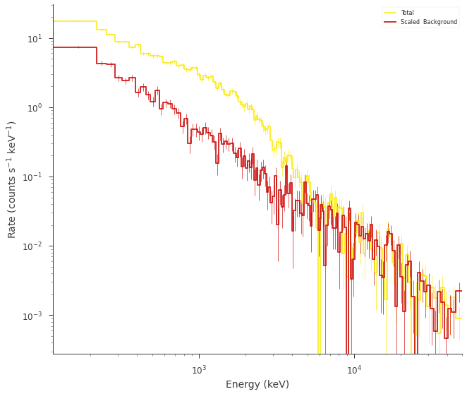
First, lets use 3ML to generate some fake data. Here we will have a background spectrum that is a power law and a source that is a black body.

Grab a demo response from the 3ML library

# we will use a demo response
response = OGIPResponse(get_path_of_data_file("datasets/ogip_powerlaw.rsp"))

Simulate the data

We will mimic the some normal c-stat style data.

np.random.seed(1234)

# rescale the functions for the response
source_function = Blackbody(K=1e-7, kT=500.0)
background_function = Powerlaw(K=1, index=-1.5, piv=1.0e3)
spectrum_generator = DispersionSpectrumLike.from_function(
    "fake",
    source_function=source_function,
    background_function=background_function,
    response=response,
)

fig = spectrum_generator.view_count_spectrum()

[INFO    ] Auto-probed noise models:
[INFO    ] - observation: poisson
[INFO    ] - background: None
[INFO    ] Auto-probed noise models:
[INFO    ] - observation: poisson
[INFO    ] - background: None
[INFO    ] Auto-probed noise models:
[INFO    ] - observation: poisson
[INFO    ] - background: poisson
[INFO    ] Auto-probed noise models:
[INFO    ] - observation: poisson
[INFO    ] - background: poisson

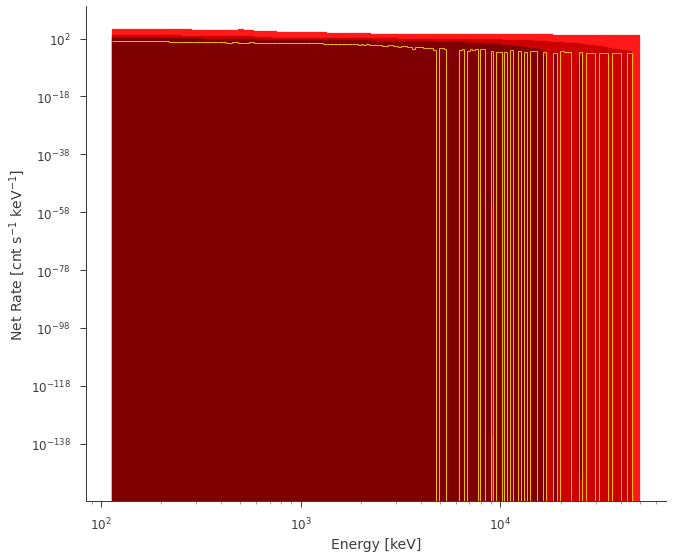
Compute the prior predictive checks

Before fitting our data, we can compute the data we would get from our prior

source_function.K.prior = Log_normal(mu=np.log(1e-7), sigma=1)
source_function.kT.prior = Log_normal(mu=np.log(300), sigma=2)

ps = PointSource("demo", 0, 0, spectral_shape=source_function)

model = Model(ps)

ba = BayesianAnalysis(model, DataList(spectrum_generator))

from twopc import compute_priorpc

ppc = compute_priorpc(
    ba, n_sims=1000, file_name="my_ppc.h5", overwrite=True, return_ppc=True
)

fig = ppc.fake.plot(bkg_subtract=True, colors=["#FF1919", "#CC0000", "#7F0000"])

Fit the data

We will quickly fit the data via Bayesian posterior sampling… After all you need a posterior to do posterior predictive checks!

ba.set_sampler("emcee")
ba.sampler.setup(n_iterations=1000, n_walkers="50")
ba.sample(quiet=False)

Maximum a posteriori probability (MAP) point:

	result	unit
parameter
demo.spectrum.main.Blackbody.K	(9.7 +/- 0.5) x 10^-8	1 / (cm2 keV3 s)
demo.spectrum.main.Blackbody.kT	(5.06 +/- 0.08) x 10^2	keV

Values of -log(posterior) at the minimum:

	-log(posterior)
fake	-631.515683
total	-631.515683

Values of statistical measures:

	statistical measures
AIC	1267.127367
BIC	1272.735427
DIC	1267.002845
PDIC	1.978515

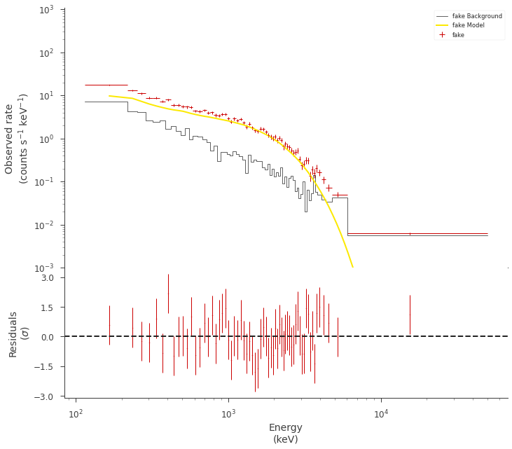
Ok, we have a pretty decent fit. But is it?

ba.restore_median_fit()
fig = display_spectrum_model_counts(
    ba,
    data_color="#CC0000",
    model_color="#FCE902",
    background_color="k",
    show_background=True,
    source_only=False,
    min_rate=10,
)
ax = fig.get_axes()[0]

_ = ax.set_ylim(1e-3)

WARNING MatplotlibDeprecationWarning: The 'nonposy' parameter of __init__() has been renamed 'nonpositive' since Matplotlib 3.3; support for the old name will be dropped two minor releases later.

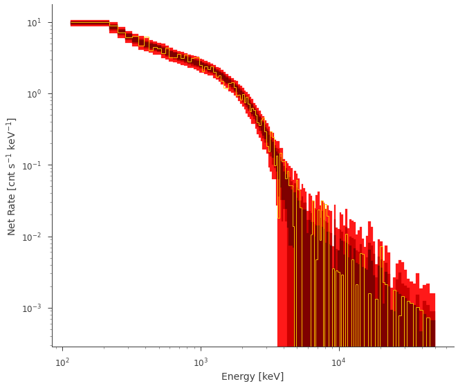
Compute the posterior predictive checks

We want to check the validiity of the fit via posterior predicitive checks (PPCs). Essentially:

\[\pi\left(y^{\mathrm{rep}} \mid y\right)=\int \mathrm{d} \theta \pi(\theta \mid y) \pi\left(y^{\mathrm{rep}} \mid \theta\right)\]

So, we will randomly sample the posterior, fold those point of the posterior model throught the likelihood and sample new counts. As this is an expensive process, we will want to save this to disk (in an HDF5 file).

from twopc import compute_postpc

ppc = compute_postpc(
    ba, ba.results, n_sims=1000, file_name="my_ppc.h5", overwrite=True, return_ppc=True
)

Lets take a look at the results of the background substracted rate

fig = ppc.fake.plot(bkg_subtract=True, colors=["#FF1919", "#CC0000", "#7F0000"])

And the PPCs with source + background

fig = ppc.fake.plot(bkg_subtract=False, colors=["#FF1919", "#CC0000", "#7F0000"])

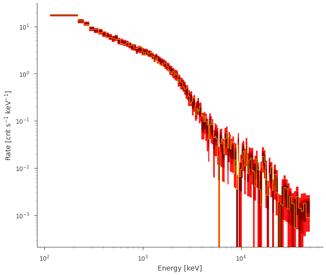
** AWESOME! ** It looks like our fit and accurately produce future data!