Localization with RBallLike

rball provides a 3ML plugin that can perform localization of point sources.

First we need to read in the database.

from astromodels import Powerlaw, PointSource, Model, Log_uniform_prior, Uniform_prior
from threeML import BayesianAnalysis, DataList


from rball import ResponseDatabase, RBallLike
from rball.utils import get_path_of_data_file
import h5py

%matplotlib inline

[WARNING ] The naima package is not available. Models that depend on it will not be available
[WARNING ] The GSL library or the pygsl wrapper cannot be loaded. Models that depend on it will not be available.
[WARNING ] The ebltable package is not available. Models that depend on it will not be available
[INFO    ] Starting 3ML!
[WARNING ] no display variable set. using backend for graphics without display (agg)
[INFO    ] Starting 3ML!
[WARNING ] no display variable set. using backend for graphics without display (agg)
[WARNING ] ROOT minimizer not available
[WARNING ] Multinest minimizer not available
[WARNING ] PyGMO is not available
[WARNING ] The cthreeML package is not installed. You will not be able to use plugins which require the C/C++ interface (currently HAWC)
[WARNING ] Could not import plugin HAWCLike.py. Do you have the relative instrument software installed and configured?
[WARNING ] Could not import plugin FermiLATLike.py. Do you have the relative instrument software installed and configured?
[WARNING ] No fermitools installed
[WARNING ] Env. variable OMP_NUM_THREADS is not set. Please set it to 1 for optimal performances in 3ML
[WARNING ] Env. variable MKL_NUM_THREADS is not set. Please set it to 1 for optimal performances in 3ML
[WARNING ] Env. variable NUMEXPR_NUM_THREADS is not set. Please set it to 1 for optimal performances in 3ML

file_name = get_path_of_data_file("demo_rsp_database.h5")

with h5py.File(file_name, "r") as f:

    # the base grid point matrices
    # should be an (N grid points, N ebounds, N monte carlo energies)
    # numpy array

    list_of_matrices = f["matrix"][()]

    # theta and phi are the
    # lon and lat points of
    # the matrix database in radian

    theta = f["theta"][()]

    phi = f["phi"][()]

    # the bounds of the response

    ebounds = f["ebounds"][()]

    mc_energies = f["mc_energies"][()]

    rsp_db = ResponseDatabase(
        list_of_matrices=list_of_matrices,
        theta=theta,
        phi=phi,
        ebounds=ebounds,
        monte_carlo_energies=mc_energies,
    )

We can create an RBallLike from normal PHA files. We will use a simulated spectrum that comes from a position on the sky (RA: 150 Dec: 0) with a power law spectrum.

demo_plugin = RBallLike.from_ogip(
    "demo",
    observation=get_path_of_data_file("demo.pha"),
    spectrum_number=1,
    response_database=rsp_db,
)

[INFO    ] Auto-probed noise models:
[INFO    ] - observation: poisson
[INFO    ] - background: None
[INFO    ] Auto-probed noise models:
[INFO    ] - observation: poisson
[INFO    ] - background: None

Fitting for the localization

We will create a 3ML point source and assign priors to the spectral parameters. The RBallLike plugin automatically assigns uniform spherical priors to the sky position. This can always be altered in the model

source_function = Powerlaw(K=1, index=-2, piv=100)

source_function.K.prior = Log_uniform_prior(lower_bound=1e-1, upper_bound=1e1)
source_function.index.prior = Uniform_prior(lower_bound=-4, upper_bound=0)

ps = PointSource("ps", 150.0, 1.0, spectral_shape=source_function)

model = Model(ps)

ba = BayesianAnalysis(model, DataList(demo_plugin))

[INFO    ] freeing the position of demo and setting priors

model

Model summary:

	N
Point sources	1
Extended sources	0
Particle sources	0

Free parameters (4):

	value	min_value	max_value	unit
ps.position.ra	150.0	0.0	360.0	deg
ps.position.dec	1.0	-90.0	90.0	deg
ps.spectrum.main.Powerlaw.K	1.0	0.0	1000.0	keV-1 s-1 cm-2
ps.spectrum.main.Powerlaw.index	-2.0	-10.0	10.0

Fixed parameters (2):
(abridged. Use complete=True to see all fixed parameters)


Linked parameters (0):

(none)

Independent variables:

(none)

Now we can sample the spectrum and position to do the localization.

ba.set_sampler("emcee")
ba.sampler.setup(n_walkers=50, n_iterations=1000.0, n_burnin=1000)

[INFO    ] sampler set to emcee

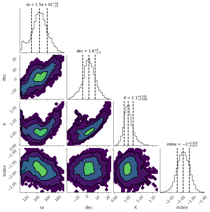
ba.sample()

[INFO    ] Mean acceptance fraction: 0.47888000000000003
Maximum a posteriori probability (MAP) point:

	result	unit
parameter
ps.position.ra	(1.45 -0.15 +0.14) x 10^2	deg
ps.position.dec	2 +/- 6	deg
ps.spectrum.main.Powerlaw.K	1.07 +/- 0.05	1 / (cm2 keV s)
ps.spectrum.main.Powerlaw.index	-1.989 -0.027 +0.028

Values of -log(posterior) at the minimum:

	-log(posterior)
demo	-407.673085
total	-407.673085

Values of statistical measures:

	statistical measures
AIC	823.671373
BIC	834.754291
DIC	819.702377
PDIC	0.011766

ba.results.corner_plot()

WARNING MatplotlibDeprecationWarning: You are modifying the state of a globally registered colormap. This has been deprecated since 3.3 and in 3.6, you will not be able to modify a registered colormap in-place. To remove this warning, you can make a copy of the colormap first. cmap = mpl.cm.get_cmap("viridis").copy()