Stellar Mass-Luminosity Bias

Suppose that stars have a mass-luminosity relationship such that \(L \propto M^3\). If we have a flux-limited survey, it will bias us towards observing more massive stars which are not representative of the full mass distribution. Let’s see how to set this up in popsynth.

Setup the problem

First, we will assume that we have some initial mass function (IMF) for our stars that describes how there masses are distributed. For simplicity, we will assume that this IMF is just a log-normal distribution:

%matplotlib inline

import matplotlib.pyplot as plt
from jupyterthemes import jtplot

jtplot.style(context="notebook", fscale=1, grid=False)
purple = "#B833FF"
yellow = "#F6EF5B"

import networkx as nx
import numpy as np
import warnings

warnings.simplefilter("ignore")

import popsynth

# create a sampler for mass
# we do not directly observe the mass as it is a latent quantity

initial_mass_function = popsynth.LogNormalAuxSampler(name="mass", observed = False)

We now assume the dependent variable is the luminosity, so we need a DerivedLumAuxSampler that generates luminosities given a mass:

class MassLuminosityRelation(popsynth.DerivedLumAuxSampler):
    _auxiliary_sampler_name = "MassLuminosityRelation"

    def __init__(self, mu=0.0, tau=1.0, sigma=1):
        # this time set observed=True
        super(MassLuminosityRelation, self).__init__("mass_lum_relation", uses_distance=False)

    def true_sampler(self, size):

            # the secondary quantity is mass

        mass = self._secondary_samplers["mass"].true_values

            # we will store the log of mass cubed
        self._true_values = 3 * np.log10(mass)

    def compute_luminosity(self):
        # compute the luminosity
            # from the relation
        return np.power(10., self._true_values)


luminosity = MassLuminosityRelation()

Now we can put everything together. First, we need to assign mass as a secondary quantity to the luminosity

luminosity.set_secondary_sampler(initial_mass_function)

Finally, we will use a simple spherical geometry to hold our stars. We will also put a hard flux limit on our survey to simulate a flux-limited catalog.

pop_gen = popsynth.populations.SphericalPopulation(1, r_max=10)

# create the flux selection

flux_selector = popsynth.HardFluxSelection()
flux_selector.boundary = 1e-2
pop_gen.set_flux_selection(flux_selector)

# now add the luminisity sampler

pop_gen.add_observed_quantity(luminosity)

Now let’s draw our survey.

pop = pop_gen.draw_survey(flux_sigma=0.5)

We can now look at the distribution of the masses:

fig, ax = plt.subplots()

bins = np.linspace(0,20,50)

ax.hist(pop.mass,
        bins=bins,
        label='all',
        color=purple,
        histtype="step",
        lw=2

       )

ax.hist(pop.mass[pop.selection],
        bins=bins,
        label='selected',
        color=yellow,
        histtype="step",
        lw=2
       )

ax.set_xlabel('stellar mass')
ax.legend()

<matplotlib.legend.Legend at 0x7feb7ce83250>

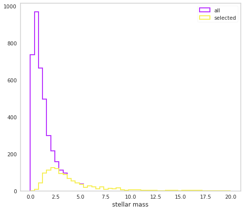
We can see that indeed our selected masses are biased towards higher values.

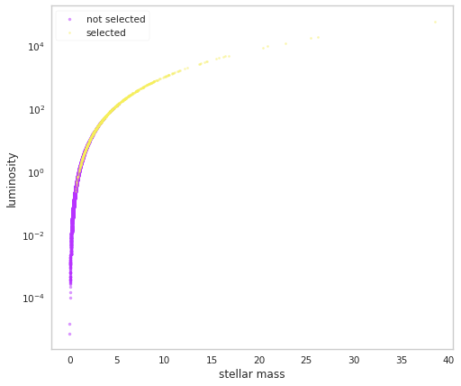
Let’s look in the mass-luminostiy plane:

fig, ax = plt.subplots()

bins = np.linspace(0,20,50)

ax.scatter(pop.mass[~pop.selection],
           pop.luminosities_latent[~pop.selection],
           label='not selected',
           color=purple,
           alpha=0.5,
           s=10



       )

ax.scatter(pop.mass[pop.selection],
           pop.luminosities_latent[pop.selection],
           label='selected',
           color=yellow,
           alpha=0.5,
           s=5
          )



ax.set_xlabel('stellar mass')
ax.set_ylabel('luminosity')
ax.set_yscale('log')


ax.legend()

<matplotlib.legend.Legend at 0x7feb79aa1eb0>